Amazon Sales Performance Dashboard
Home // AI-Powered Data Analysis
📋 Project Overview
 Objective:
The goal of this project is to analyze Amazon sales data to uncover key insights about sales performance, customer behavior, and operational efficiency. I used statistical methods to identify trends, relationships, and factors influencing sales outcomes.
Key Analyses & Methods:
 Descriptive Statistics (Data Summary)
- Analyze sales distribution (total revenue, order count, average order value).
- Identify top-selling categories and products.
- Examine order status breakdown (shipped, canceled, returned).
Inferential Statistics (Comparisons & Hypothesis Testing)
- T-test/ANOVA: Compare sales performance between B2B vs. B2C and fulfillment methods.
- Chi-Square Test: Analyze relationships between order status and fulfillment methods.
- Correlation Analysis: Identify relationships between
QtyandAmount.
Time Series & Trend Analysis
- Identify monthly and seasonal sales trends.
Outlier Detection & Data Quality Checks
- Detect unusual patterns in order amounts using boxplots & statistical methods.
- Handle missing values and anomalies for better data reliability.
Expected Outcomes:
- Actionable insights into revenue trends, high-performing categories, and sales channels.
- Statistical evidence of key sales-driving factors (B2B vs. B2C, fulfillment method impact).
📚 Workflow
✅Data Preprocessing
- Load & Inspect: Check data structure, types, and missing values.
- Clean Data: Handle missing values, convert dates, and standardize categories.
- Detect Outliers: Use boxplots, Z-score, and IQR methods.
✅Descriptive Statistics & Sales Analysis
- Overall Sales: Total revenue, order count, average order value.
- Category & Product Analysis: Identify top-selling items.
- Order Status: Shipped vs. Canceled impact on revenue.
- Fulfillment & B2B vs. B2C: Compare sales performance.
✅Statistical Analysis & Hypothesis Testing
- T-Test/ANOVA: Compare B2B vs. B2C and category sales.
- Chi-Square: Test relationships (e.g., Order Status vs. Fulfillment).
- Correlation & Regression: Analyze
Qtyvs.Amount, build predictive models.
✅Time Series & Trend Analysis
- Sales Trends: Monthly & seasonal revenue insights.
- Forecasting (Optional): Predict future sales using time series models.
✅Data Visualization & Insights
- Charts & Graphs: Revenue trends, sales distribution, fulfillment comparisons.
- Insights & Recommendations: Summarize key findings for decision-making.
✅Dashboard
- Report: Document key metrics & trends.
- Power BI Dashboard: Create interactive visuals for easy insights.
📊 Summary of the Dataset
📊 Summary of the Amazon Sales Dataset
- Dataset Name: Amazon Sales Data
- Total Rows: 128,976
- Total Columns: 19
🔑 Key Columns & Descriptions:
index – Row index (not necessary for analysis).- order_id – Unique identifier for each order.
- date – Date of the order.
- status – Current status of the order (Shipped, Cancelled, etc.).
- fulfilment – Whether fulfilled by Amazon or Merchant.
- sales_channel – Platform where the sale was made.
- ship_service_level – Type of shipping service selected.
- category – Product category.
- size – Product size.
- courier_status – Delivery status from the courier.
- qty – Quantity of items in the order.
- currency – Currency used for the order.
- amount – Total sales amount for the order.
- ship_city – Destination city of the order.
- ship_state – Destination state of the order.
- ship_postal_code – Postal code of the shipping address.
- ship_country – Destination country of the order.
- b2b – Whether the order is Business-to-Business (B2B) or not.
- fulfilled_by – Fulfillment method used (Amazon, Merchant, etc.).
🗂️ Data Processing
Drop Columns
					# Drop unnecessary columns: 'index' and 'ship_postal_code'
df.drop(columns=['index', 'ship_postal_code'], inplace=True)
Remove Duplicates
					# Check for duplicate rows
duplicate_count = df.duplicated().sum()

# Remove duplicate rows
df.drop_duplicates(inplace=True)

# Verify if duplicates remain
remaining_duplicates = df.duplicated().sum()

# Display results
duplicate_summary = {
    "Duplicates Found": duplicate_count,
    "Duplicates Removed": duplicate_count,
    "Remaining Duplicates": remaining_duplicates
}
					{'Duplicates Found': np.int64(168),
 'Duplicates Removed': np.int64(168),
 'Remaining Duplicates': np.int64(0)}
Handling Missing Values
| Missing Values | Percentage (%) | |
|---|---|---|
| fulfilled_by | 89713 | 70.0 |
| currency | 7800 | 6.0 |
| amount | 7800 | 6.0 |
| ship_postal_code | 35 | 0.0 |
| ship_country | 35 | 0.0 |
| ship_state | 35 | 0.0 |
| ship_city | 35 | 0.0 |
					# Check for missing values in each column
missing_values = df.isnull().sum()
missing_percentage = round((missing_values / df.shape[0]) * 100)

# Create a summary DataFrame for missing values
missing_summary = pd.DataFrame({
    "Missing Values": missing_values,
    "Percentage (%)": missing_percentage
}).sort_values(by="Missing Values", ascending=False)

# Display columns with missing values
missing_summary[missing_summary["Missing Values"] > 0]
					# Fill NaN values in 'fulfilled-by' with 'Merchant Fulfilled'
df['fulfilled_by'].fillna("Merchant Fulfilled", inplace=True)

# Verify the changes
df['fulfilled_by'].unique()
array(['Easy Ship', 'Merchant Fulfilled'], dtype=object)
					# Fill missing 'Amount' values with 0 for cancelled orders
df.loc[(df['amount'].isnull()) & (df['courier_status'] == 'Cancelled'), 'amount'] = 0
					# Calculate the median of 'amount' (excluding 0 values)
median_amount = df[df['amount'] > 0]['amount'].median()

# Fill missing 'amount' for shipped & unshipped orders with the median
df.loc[(df['amount'].isnull()) & (df['status'] == 'Shipped') & (df['courier_status'] == 'Unshipped'), 'amount'] = median_amount

# Fill missing 'amount' for Shipped - Delivered to Buyer & on the way orders with the median
df.loc[(df['amount'].isnull()) & (df['status'] == 'Shipped - Delivered to Buyer') & (df['courier_status'] == 'On the Way'), 'amount'] = median_amount

# Fill missing 'amount' for Shipped - Returned to Seller & On the Way orders with the median
df.loc[(df['amount'].isnull()) & (df['status'] == 'Shipped - Returned to Seller') & (df['courier_status'] == 'On the Way'), 'amount'] = median_amount

# Fill missing 'amount' for Shipping & Unshipped orders with the median
df.loc[(df['amount'].isnull()) & (df['status'] == 'Shipping') & (df['courier_status'] == 'Unshipped'), 'amount'] = median_amount

# Fill missing 'amount' for Cancelled & Unshipped with the 0
df.loc[(df['amount'].isnull()) & (df['status'] == 'Cancelled') & (df['courier_status'] == 'Unshipped'), 'amount'] = 0

# Fill missing 'amount' for cancelled & on the way orders with 0
df.loc[(df['amount'].isnull()) & (df['status'] == 'Cancelled') & (df['courier_status'] == 'On the Way'), 'amount'] = 0
					# Fill missing 'currency' values with 'INR' (since only one country is present)
df['currency'].fillna('INR', inplace=True)
					# Fill missing values in ship_city, ship_state, and ship_postal_code with 'Unknown'
df['ship_city'].fillna('Unknown', inplace=True)
df['ship_state'].fillna('Unknown', inplace=True)
df['ship_postal_code'].fillna('Unknown', inplace=True)

# Fill missing values in ship_country with 'IN' (since only one country is present)
df['ship_country'].fillna('IN', inplace=True)
df.isna().sum()
					index                 0
order_id              0
date                  0
status                0
fulfilment            0
sales_channel         0
ship_service_level    0
category              0
size                  0
courier_status        0
qty                   0
currency              0
amount                0
ship_city             0
ship_state            0
ship_postal_code      0
ship_country          0
b2b                   0
fulfilled_by          0
dtype: int64
Standardizing Column Names
					#  Standardizing column names with lowercase and underscores

df.columns = df.columns.str.replace(' ', '_')
df.columns = df.columns.str.replace('-', '_')
df.columns = df.columns.str.lower()
					Index(['index', 'order_id', 'date', 'status', 'fulfilment', 'sales_channel',
       'ship_service_level', 'category', 'size', 'courier_status', 'qty',
       'currency', 'amount', 'ship_city', 'ship_state', 'ship_postal_code',
       'ship_country', 'b2b', 'fulfilled_by'],
      dtype='object')
Data Type Conversion
					# Check the current data types of all columns
df.dtypes
					index                   int64
order_id               object
date                   object
status                 object
fulfilment             object
sales_channel          object
ship_service_level     object
category               object
size                   object
courier_status         object
qty                     int64
currency               object
amount                float64
ship_city              object
ship_state             object
ship_postal_code       object
ship_country           object
b2b                      bool
fulfilled_by           object
dtype: object
					# Convert 'date' to datetime format
df['date'] = pd.to_datetime(df['date'], errors='coerce')
					# Get unique values count for each categorical column
categorical_columns = [
    'status', 'fulfilment', 'sales_channel', 'ship_service_level',
    'category', 'size', 'courier_status', 'ship_country', 'fulfilled_by'
]

unique_values_summary = {col: df[col].nunique() for col in categorical_columns}
unique_values_summary
					{'status': 13,
 'fulfilment': 2,
 'sales_channel': 2,
 'ship_service_level': 2,
 'category': 9,
 'size': 11,
 'courier_status': 4,
 'ship_country': 1,
 'fulfilled_by': 2}
df['status'].unique()
					array(['Cancelled', 'Shipped - Delivered to Buyer', 'Shipped',
       'Shipped - Returned to Seller', 'Shipped - Rejected by Buyer',
       'Shipped - Lost in Transit', 'Shipped - Out for Delivery',
       'Shipped - Returning to Seller', 'Shipped - Picked Up', 'Pending',
       'Pending - Waiting for Pick Up', 'Shipped - Damaged', 'Shipping'],
      dtype=object)
					# Define a mapping dictionary to simplify 'status' values
status_mapping = {
    "Cancelled": "Cancelled",
    "Pending": "Pending",
    "Pending - Waiting for Pick Up": "Pending",
    "Shipped": "Shipped",
    "Shipped - Delivered to Buyer": "Delivered",
    "Shipped - Out for Delivery": "Out for Delivery",
    "Shipped - Picked Up": "Picked Up",
    "Shipped - Returned to Seller": "Returned",
    "Shipped - Returning to Seller": "Returned",
    "Shipped - Rejected by Buyer": "Returned",
    "Shipped - Lost in Transit": "Lost/Damaged",
    "Shipped - Damaged": "Lost/Damaged",
    "Shipping": "Shipped"
}

# Apply the mapping
df['status'] = df['status'].map(status_mapping)

# Verify the updated unique values
df['status'].unique()
					array(['Cancelled', 'Delivered', 'Shipped', 'Returned', 'Lost/Damaged',
       'Out for Delivery', 'Picked Up', 'Pending'], dtype=object)
					# Convert categorical columns to 'category' data type
categorical_columns = [
    'status', 'fulfilment', 'sales_channel', 'ship_service_level',
    'category', 'size', 'courier_status', 'ship_country', 'fulfilled_by'
]

for col in categorical_columns:
    df[col] = df[col].astype('category')

# Verify the changes
df.dtypes
					index                   int64
order_id               object
date                   object
status                 object
fulfilment             object
sales_channel          object
ship_service_level     object
category               object
size                   object
courier_status         object
qty                     int64
currency               object
amount                float64
ship_city              object
ship_state             object
ship_postal_code       object
ship_country           object
b2b                      bool
fulfilled_by           object
dtype: object
					index                          int64
order_id                      object
date                  datetime64[ns]
status                      category
fulfilment                  category
sales_channel               category
ship_service_level          category
category                    category
size                        category
courier_status              category
qty                            int64
currency                      object
amount                       float64
ship_city                     object
ship_state                    object
ship_postal_code              object
ship_country                category
b2b                             bool
fulfilled_by                category
dtype: object
Outlier Detection & Handling
					import numpy as np

# Function to detect outliers using IQR
def detect_outliers_iqr(data, column):
    Q1 = np.percentile(data[column], 25)  # First quartile
    Q3 = np.percentile(data[column], 75)  # Third quartile
    IQR = Q3 - Q1  # Interquartile range
    lower_bound = Q1 - 1.5 * IQR
    upper_bound = Q3 + 1.5 * IQR

    outliers = data[(data[column] < lower_bound) | (data[column] > upper_bound)]
    return outliers.shape[0], lower_bound, upper_bound

# Detect outliers in 'qty' and 'amount'
qty_outliers, qty_lower, qty_upper = detect_outliers_iqr(df, 'qty')
amount_outliers, amount_lower, amount_upper = detect_outliers_iqr(df, 'amount')

# Create a summary DataFrame
outlier_summary = pd.DataFrame({
    "Column": ["qty", "amount"],
    "Outlier Count": [qty_outliers, amount_outliers],
    "Lower Bound": [qty_lower, amount_lower],
    "Upper Bound": [qty_upper, amount_upper]
})

outlier_summary
| Column | Outlier Count | Lower Bound | Upper Bound |
|---|---|---|---|
| qty | 13179 | 1.0 | 1.0 |
| amount | 3174 | -116.5 | 1303.5 |
					# Flag outliers in 'amount' based on IQR bounds
amount_lower_bound = -116.5  # From IQR summary
amount_upper_bound = 1303.5

df['amount_outlier'] = ((df['amount'] < amount_lower_bound) | (df['amount'] > amount_upper_bound))

# Verify how many outliers were flagged
df['amount_outlier'].sum()
np.int64(3174)
					from scipy import stats

# Calculate Z-scores for 'amount'
df['amount_zscore'] = stats.zscore(df['amount'], nan_policy='omit')

# Flag outliers using Z-score (threshold ±3)
df['amount_outlier_z'] = df['amount_zscore'].abs() > 3

# Count the number of Z-score flagged outliers
zscore_outliers_count = df['amount_outlier_z'].sum()

zscore_outliers_count
np.int64(439)
					# Keep the outliers but flag them instead of removing
df['amount_outlier'] = df['amount_zscore'].abs() > 3

# Drop only temporary Z-score columns
df.drop(columns=['amount_zscore','amount_outlier_z'], inplace=True)
Validation
					# Final Data Validation

total_rows, total_columns = df.shape
remaining_missing_values = df.isnull().sum().sum()
outlier_count = df['amount_outlier'].sum()
duplicate_count = df.duplicated().sum()

# Create summary dataframe
final_summary = pd.DataFrame({
    "Total Rows": [total_rows],
    "Total Columns": [total_columns],
    "Remaining Missing Values": [remaining_missing_values],
    "Flagged Amount Outliers": [outlier_count],
    "duplicate_count": [duplicate_count]
})
final_summary
| Total Rows | Total Columns | Remaining Missing Values | Flagged Amount Outliers | duplicate_count |
|---|---|---|---|---|
| 128808 | 20 | 0 | 439 | 0 |
💾 Descriptive Statistics & Sales Analysis
Overall Sales Summary
					# Compute overall sales summary by status
overall_sales_summary = df.groupby('status').agg({
    'amount': ['sum', 'mean', 'median','min','max'],
    'qty': ['sum', 'mean', 'median','min','max']
})

# Compute correct "Grand Total" values separately
grand_total_values = {
    ('amount', 'sum'): df['amount'].sum(),
    ('amount', 'mean'): df['amount'].mean(),
    ('amount', 'median'): df['amount'].median(),
    ('qty', 'sum'): df['qty'].sum(),
    ('qty', 'mean'): df['qty'].mean(),
    ('qty', 'median'): df['qty'].median()
}

# Convert to DataFrame and append as "Grand Total" row
grand_total = pd.DataFrame([grand_total_values], index=["Grand Total"])
overall_sales_summary = pd.concat([overall_sales_summary, grand_total])

overall_sales_summary
| amount | amount | amount | amount | amount | qty | qty | qty | qty | qty | |
|---|---|---|---|---|---|---|---|---|---|---|
| sum | mean | median | min | max | sum | mean | median | min | max | |
| Cancelled | 6910831.39 | 377.41419856916605 | 380.0 | 0.0 | 4235.72 | 5651 | 0.3086123095407132 | 0.0 | 0.0 | 2.0 |
| Delivered | 18624586.0 | 648.6012885251611 | 631.0 | 0.0 | 5495.0 | 28831 | 1.0040397005049626 | 1.0 | 0.0 | 5.0 |
| Lost/Damaged | 3133.0 | 522.1666666666666 | 499.0 | 0.0 | 1136.0 | 6 | 1.0 | 1.0 | 1.0 | 1.0 |
| Out for Delivery | 26971.0 | 770.6 | 729.0 | 301.0 | 1399.0 | 35 | 1.0 | 1.0 | 1.0 | 1.0 |
| Pending | 622409.0 | 662.842385516507 | 664.0 | 0.0 | 2326.0 | 940 | 1.0010649627263046 | 1.0 | 0.0 | 2.0 |
| Picked Up | 661252.0 | 679.601233299075 | 699.0 | 0.0 | 1998.0 | 977 | 1.0041109969167523 | 1.0 | 1.0 | 2.0 |
| Returned | 1386026.0 | 657.5075901328273 | 635.0 | 0.0 | 2796.0 | 2130 | 1.0104364326375712 | 1.0 | 0.0 | 4.0 |
| Shipped | 50344926.0 | 647.7647739993052 | 599.0 | 0.0 | 5584.0 | 77926 | 1.002637639762741 | 1.0 | 0.0 | 15.0 |
| Grand Total | 78580134.39000002 | 610.056319405627 | 588.0 | 116496 | 0.9044158747903857 | 1.0 |
Category & Product Analysis
					# Compute category sales summary
category_sales_summary = df.groupby('category').agg({
    'amount': ['sum', 'mean', 'median', 'min', 'max'],
    'qty': ['sum', 'mean', 'median', 'min', 'max']
}).sort_values(('amount', 'sum'), ascending=False)

category_sales_summary
| amount | amount | amount | amount | amount | qty | qty | qty | qty | qty | |
|---|---|---|---|---|---|---|---|---|---|---|
| sum | mean | median | min | max | sum | mean | median | min | max | |
| category | ||||||||||
| T-shirt | 39193318.17 | 780.4480011549414 | 759.0 | 0.0 | 5584.0 | 45228 | 0.9006153049642566 | 1.0 | 0 | 8 |
| Shirt | 21304600.7 | 427.7688679624126 | 432.0 | 0.0 | 2796.0 | 44978 | 0.9031001525981849 | 1.0 | 0 | 13 |
| Blazzer | 11211616.12 | 723.8437678352378 | 744.0 | 0.0 | 2860.0 | 13934 | 0.8996061721221512 | 1.0 | 0 | 4 |
| Trousers | 5344415.3 | 503.85738663146975 | 518.0 | 0.0 | 1797.0 | 9889 | 0.93230885264448 | 1.0 | 0 | 3 |
| Perfume | 789419.66 | 682.2987554019015 | 797.14 | 0.0 | 1449.0 | 1051 | 0.9083837510803803 | 1.0 | 0 | 2 |
| Wallet | 460896.18 | 497.72805615550755 | 518.525 | 0.0 | 1266.66 | 863 | 0.9319654427645788 | 1.0 | 0 | 15 |
| Socks | 151019.5 | 344.0079726651481 | 342.86 | 0.0 | 1028.58 | 398 | 0.9066059225512528 | 1.0 | 0 | 2 |
| Shoes | 123933.76 | 755.6936585365853 | 790.0 | 0.0 | 2058.0 | 152 | 0.926829268292683 | 1.0 | 0 | 3 |
| Watch | 915.0 | 305.0 | 305.0 | 305.0 | 305.0 | 3 | 1.0 | 1.0 | 1 | 1 |
					# Compute sales summary by product
product_sales_summary = df.groupby('size').agg({
    'amount': ['sum', 'mean', 'median', 'min', 'max'],
    'qty': ['sum', 'mean', 'median', 'min', 'max']
}).sort_values(('amount', 'sum'), ascending=False)

product_sales_summary
| amount | amount | amount | amount | amount | qty | qty | qty | qty | qty | |
|---|---|---|---|---|---|---|---|---|---|---|
| sum | mean | median | min | max | sum | mean | median | min | max | |
| size | ||||||||||
| M | 13691357.13 | 612.5886859060403 | 597.0 | 0.0 | 4235.72 | 20116 | 0.9000447427293065 | 1.0 | 0 | 4 |
| L | 13038244.84 | 598.7162988474078 | 573.0 | 0.0 | 2598.0 | 19680 | 0.9037057445929191 | 1.0 | 0 | 9 |
| XL | 12255023.38 | 597.2233615984405 | 563.0 | 0.0 | 2698.0 | 18609 | 0.9068713450292397 | 1.0 | 0 | 5 |
| XXL | 10461329.64 | 588.2769858853962 | 545.0 | 0.0 | 2676.0 | 16226 | 0.9124444694371029 | 1.0 | 0 | 13 |
| S | 10426761.18 | 622.3445851736899 | 599.0 | 0.0 | 2864.0 | 15022 | 0.8966217022800526 | 1.0 | 0 | 4 |
| 3XL | 9034190.92 | 617.6802215233147 | 581.0 | 0.0 | 5495.0 | 13346 | 0.9124846164364829 | 1.0 | 0 | 5 |
| XS | 6960339.1 | 630.8655034895314 | 622.86 | 0.0 | 5584.0 | 9829 | 0.8908728360373425 | 1.0 | 0 | 8 |
| Free | 1375164.6 | 611.1842666666668 | 625.0 | 0.0 | 2058.0 | 2069 | 0.9195555555555556 | 1.0 | 0 | 15 |
| 6XL | 577493.33 | 782.5112872628725 | 798.0 | 0.0 | 1672.0 | 688 | 0.9322493224932249 | 1.0 | 0 | 2 |
| 5XL | 425778.63 | 774.1429636363637 | 798.0 | 0.0 | 1629.0 | 513 | 0.9327272727272727 | 1.0 | 0 | 2 |
| 4XL | 334451.64 | 783.2591100702576 | 798.0 | 0.0 | 1672.0 | 398 | 0.9320843091334895 | 1.0 | 0 | 2 |
Fulfillment & B2B vs. B2C Analysis
					# Compute sales summary by fulfillment method
fulfillment_summary = df.groupby('fulfilled_by').agg({
    'amount': ['sum', 'mean', 'median', 'min', 'max'],
    'qty': ['sum', 'mean', 'median', 'min', 'max']
}).sort_values(('amount', 'sum'), ascending=False)

# Compute sales summary by B2B vs. B2C
b2b_summary = df.groupby('b2b').agg({
    'amount': ['sum', 'mean', 'median', 'min', 'max'],
    'qty': ['sum', 'mean', 'median', 'min', 'max']
}).sort_values(('amount', 'sum'), ascending=False)

b2b_summary
fulfillment_summary
| amount | amount | amount | amount | amount | qty | qty | qty | qty | qty | |
|---|---|---|---|---|---|---|---|---|---|---|
| sum | mean | median | min | max | sum | mean | median | min | max | |
| b2b | ||||||||||
| False | 77988913.6 | 609.5884193001242 | 587.0 | 0.0 | 5584.0 | 115656 | 0.9040074411624471 | 1.0 | 0 | 15 |
| True | 591220.79 | 678.7839150401837 | 653.0 | 0.0 | 5495.0 | 840 | 0.9644087256027555 | 1.0 | 0 | 5 |
| amount | amount | amount | amount | amount | qty | qty | qty | qty | qty | |
|---|---|---|---|---|---|---|---|---|---|---|
| sum | mean | median | min | max | sum | mean | median | min | max | |
| fulfilled_by | ||||||||||
| Merchant Fulfilled | 54338671.0 | 606.4922261286902 | 574.0 | 0.0 | 5584.0 | 83990 | 0.9374407053965065 | 1.0 | 0 | 15 |
| Easy Ship | 24241463.39 | 618.1996631219239 | 602.86 | 0.0 | 5495.0 | 32506 | 0.8289597837451865 | 1.0 | 0 | 5 |
♟Statistical Analysis & Hypothesis Testing
T-Test/ANOVA for B2B vs. B2C and Category Sales Comparisons
					from scipy.stats import ttest_ind, f_oneway

# T-Test for B2B vs. B2C Sales Comparison
b2b_sales = df[df['b2b'] == True]['amount']
b2c_sales = df[df['b2b'] == False]['amount']

# Perform independent T-test
t_stat, p_value_b2b = ttest_ind(b2b_sales, b2c_sales, equal_var=False, nan_policy='omit')

# ANOVA for Category Sales Comparison
category_groups = [group['amount'].dropna() for name, group in df.groupby('category')]

# Perform ANOVA test
anova_stat, p_value_category = f_oneway(*category_groups)

# Create a summary DataFrame for hypothesis testing results
hypothesis_results = pd.DataFrame({
    "Test": ["T-Test (B2B vs. B2C)", "ANOVA (Category Sales)"],
    "Test Statistic": [t_stat, anova_stat],
    "P-Value": [p_value_b2b, p_value_category]
})

hypothesis_results
| Test | Test Statistic | P-Value | |
|---|---|---|---|
| 0 | T-Test (B2B vs. B2C) | 5.782585515575493 | 1.0216579602426602e-08 |
| 1 | ANOVA (Category Sales) | 6157.193563145301 | 0.0 |
1️⃣ T-Test (B2B vs. B2C)
Test Statistic (5.78):
- A high t-value means a strong difference between B2B and B2C sales amounts.
- This shows that the two groups have significantly different mean sales.
P-Value (1.02e-08 or 0.0000000102):
- The probability that this difference happened by random chance is almost zero.
- Since p < 0.05, we reject the null hypothesis, meaning B2B and B2C sales are significantly different.
✅ Conclusion:
- B2B sales behave differently than B2C sales in terms of order amount.
2️⃣ ANOVA (Category Sales)
Test Statistic (6157.19):
- A very high F-statistic means that there is a strong difference in sales across different categories.
P-Value (0.000):
- The probability that all categories have the same sales is almost zero.
- Since p < 0.05, we reject the null hypothesis, meaning some product categories sell significantly better than others.
✅ Conclusion:
- Product categories show significant differences in sales performance. Some categories are selling far more or far less than others.
Chi-Square Analysis (Order Status vs. Fulfillment Method)
					import scipy.stats as stats

# Create a contingency table
contingency_table = pd.crosstab(df['status'], df['fulfilled_by'])

# Perform Chi-Square test
chi2_stat, p_value_chi2, dof, expected = stats.chi2_contingency(contingency_table)

# Create a summary DataFrame for the Chi-Square test results
chi_square_results = pd.DataFrame({
    "Test": ["Chi-Square (Order Status vs. Fulfillment)"],
    "Chi-Square Statistic": [chi2_stat],
    "P-Value": [p_value_chi2],
    "Degrees of Freedom": [dof]
})
chi_square_results
| Test | Chi-Square Statistic | P-Value | Degrees of Freedom |
|---|---|---|---|
| Chi-Square (Order Status vs. Fulfillment) | 107464.38698839529 | 0.0 | 7 |
Chi-Square Statistic (107464.39)
- A very high value indicates a strong relationship between order status and fulfillment method (Amazon vs. Merchant).
- This means that order fulfillment type affects whether an order is shipped, canceled, or returned.
P-Value (0.000)
- The probability of this result happening by random chance is almost zero.
- Since p < 0.05, we reject the null hypothesis, meaning order status is significantly influenced by the fulfillment method.
Degrees of Freedom (7)
- This is based on the number of categories in
statusandfulfilled_by.
- This is based on the number of categories in
✅ Conclusion:
The fulfillment method significantly affects order status. Orders fulfilled by Amazon vs. Merchant have different cancellation, return, and shipping rates.
Correlation & Regression Analysis (Qty vs. Amount)
					# Correlation & Regression Analysis (Qty vs. Amount)
import seaborn as sns
import matplotlib.pyplot as plt
import statsmodels.api as sm

# Calculate Pearson correlation coefficient
correlation_coefficient = df['qty'].corr(df['amount'])

# Scatter plot with regression line
plt.figure(figsize=(8, 5))
sns.regplot(x=df['qty'], y=df['amount'], scatter_kws={"alpha":0.3}, line_kws={"color":"red"})
plt.xlabel("Quantity (Qty)")
plt.ylabel("Amount ($)")
plt.title(f"Correlation between Quantity and Amount (r = {correlation_coefficient:.2f})")
plt.show()

# Perform linear regression (OLS - Ordinary Least Squares)
X = sm.add_constant(df['qty'])  # Add constant for intercept
y = df['amount']
model = sm.OLS(y, X).fit()

# Display regression summary
regression_summary = model.summary()
regression_summary
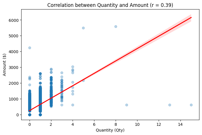
✅Correlation Coefficient (r = 0.39)
- Shows a moderate positive correlation between quantity (qty) and amount.
- Higher quantities tend to be associated with higher sales, but the relationship is not perfectly linear.
✅Regression Line (Red Line in Plot)
- The upward slope confirms a positive relationship between quantity and amount.
- Some outliers exist where low quantities still result in high sales amounts.
					OLS Regression Results
==============================================================================
Dep. Variable:                 amount   R-squared:                       0.155
Model:                            OLS   Adj. R-squared:                  0.155
Method:                 Least Squares   F-statistic:                 2.369e+04
Date:                Fri, 14 Mar 2025   Prob (F-statistic):               0.00
Time:                        17:08:52   Log-Likelihood:            -9.1196e+05
No. Observations:              128808   AIC:                         1.824e+06
Df Residuals:                  128806   BIC:                         1.824e+06
Df Model:                           1
Covariance Type:            nonrobust
==============================================================================
                 coef    std err          t      P>|t|      [0.025      0.975]
------------------------------------------------------------------------------
const        254.2724      2.446    103.941      0.000     249.478     259.067
qty          393.3853      2.556    153.920      0.000     388.376     398.395
==============================================================================
Omnibus:                    17866.214   Durbin-Watson:                   1.863
Prob(Omnibus):                  0.000   Jarque-Bera (JB):            58717.680
Skew:                           0.709   Prob(JB):                         0.00
Kurtosis:                       5.988   Cond. No.                         5.95
==============================================================================
1️⃣ Model Summary
- Dep. Variable:
amount→ This is the target variable (sales amount) we are predicting. - Model Type: OLS (Ordinary Least Squares) → The type of regression used.
- Method: Least Squares → The method used to estimate coefficients.
- No. Observations: 128,088 → The total number of data points (rows) in the dataset.
- Df Residuals: 128,086 → Degrees of freedom left after estimating model parameters.
- Df Model: 1 → The number of predictor variables in the model (
qty).
2️⃣ Model Fit Statistics (How Well the Model Explains Variance)
- R-squared: 0.155 → This means that 15.5% of the variation in
amountis explained byqty. A low R² suggests other factors influence sales. - Adjusted R-squared: 0.155 → Similar to R² but adjusted for additional predictors (remains the same since we have only one predictor).
- F-statistic: 23,690 → A high F-value indicates that the model is statistically significant.
- Prob (F-statistic): 0.000 → Since p < 0.05, the model is statistically significant.
Interpretation:
- The model has low explanatory power (R² = 15.5%), meaning
qtydoes not fully predictamount—other factors are influencing sales.
3️⃣ Regression Coefficients (How qty Affects amount)
- Intercept (const):
254.27→ Ifqty = 0, the predicted sales amount is $254.27 (base value). - Quantity (qty):
393.39→ Each additional unit sold increasesamountby $393.39 on average.
Statistical Significance of Predictors:
- Standard Error (
std err):- Measures how much the estimated coefficient might vary. Smaller values are better.
- t-statistic (
t):- Measures how strongly a variable influences the dependent variable. Higher absolute values mean stronger relationships.
- p-value (
P>|t|):- Measures statistical significance. If p < 0.05, the variable significantly affects
amount. - Both
constandqtyare statistically significant (p = 0.000).
- Measures statistical significance. If p < 0.05, the variable significantly affects
- 95% Confidence Interval:
- The range where the true coefficient likely falls.
- Example:
qtyis likely between $388.38 to $398.39 per unit increase.
Interpretation:
qtyhas a significant positive impact onamount—each unit sold increases sales by ~$393.39.
4️⃣ Residual Diagnostics (Checking Model Assumptions)
- Omnibus: 17,866.214 → Tests if residuals are normally distributed. High values suggest they are not normal.
- Prob (Omnibus): 0.000 → Residuals are not normally distributed (p < 0.05).
- Durbin-Watson: 1.863 → Measures autocorrelation (values between 1.5 – 2.5 are acceptable).
- Jarque-Bera (JB): 58,717.68 → Another normality test—high values confirm non-normal residuals.
- Prob (JB): 0.000 → Residuals fail the normality test (p < 0.05).
- Skew: 0.709 → Residuals are slightly right-skewed.
- Kurtosis: 5.988 → Residuals have heavy tails (outliers present).
- Condition Number (Cond. No.): 5.95 → Measures multicollinearity (values > 30 are problematic; this model is fine).
Interpretation:
- Residuals are not normally distributed → This suggests the model may need transformation.
- Some skewness and outliers exist → The model could be improved.
- No severe multicollinearity detected, so predictor variables are independent.
🚀 Key Takeaways:
✅ qty significantly predicts amount (p < 0.05)—each additional unit sold increases revenue by ~$393.39.
✅ The model explains 15.5% of sales variation, meaning other factors influence sales.
✅ Residuals are not normally distributed, which suggests potential model improvement (e.g., transformation).
Time Series & Trend Analysis (Sales Trends & Seasonality)
					# Aggregate sales by month to analyze trends
monthly_sales = df.resample('M', on='date').agg({'amount': 'sum'}).reset_index()

# Plot the monthly sales trend
plt.figure(figsize=(12, 6))
plt.plot(monthly_sales['date'], monthly_sales['amount'], marker='o', linestyle='-', color='b')
plt.xlabel("Month")
plt.ylabel("Total Sales Amount ($)")
plt.title("Monthly Sales Trend Over Time")
plt.grid(True)
plt.show()
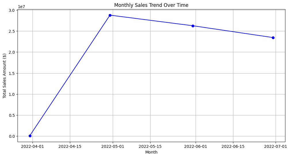
✅ Sales Growth and Decline:
- The chart shows a sharp increase in sales in April, peaking in May.
- After the peak, sales gradually decline from June to July.
✅ Possible Reasons for Trends:
- Sales Peak in May: Likely due to seasonal demand, promotions, or new product launches.
- Decline After May: Could be due to market saturation, reduced marketing, or seasonal effects.
🕒Time Series & Trend Analysis
Time Series & Trend Analysis (Sales Trends & Seasonality)
					# Aggregate sales by month to analyze trends
monthly_sales = df.resample('M', on='date').agg({'amount': 'sum'}).reset_index()

# Plot the monthly sales trend
plt.figure(figsize=(12, 6))
plt.plot(monthly_sales['date'], monthly_sales['amount'], marker='o', linestyle='-', color='b')
plt.xlabel("Month")
plt.ylabel("Total Sales Amount ($)")
plt.title("Monthly Sales Trend Over Time")
plt.grid(True)
plt.show()
✅ Sales Growth and Decline:
- The chart shows a sharp increase in sales in April, peaking in May.
- After the peak, sales gradually decline from June to July.
✅ Possible Reasons for Trends:
- Sales Peak in May: Likely due to seasonal demand, promotions, or new product launches.
- Decline After May: Could be due to market saturation, reduced marketing, or seasonal effects.
🎨Data Visualization & Insights
					import seaborn as sns

# Create a bar chart for sales by category
plt.figure(figsize=(12, 6))
sns.barplot(x=df.groupby('category')['amount'].sum().index,
            y=df.groupby('category')['amount'].sum().values,
            palette="viridis")

plt.xlabel("Product Category")
plt.ylabel("Total Sales Amount ($)")
plt.title("Total Sales by Product Category")
plt.xticks(rotation=45)
plt.grid(axis='y', linestyle='--', alpha=0.7)
plt.show()
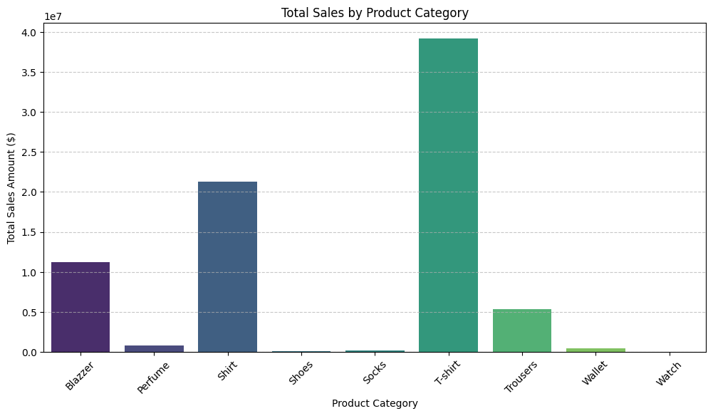
🔎 Key Insights:
1️⃣ T-Shirts Dominate Sales
- Highest-selling category with total sales nearing 40 million.
- Suggests high demand or strong marketing efforts for T-shirts.
2️⃣ Shirts and Blazers Perform Well
- Shirts (~21 million) and Blazers (~11 million) contribute significantly to revenue.
- Indicates consistent demand for formal/casual wear.
3️⃣ Low-Selling Categories (Shoes, Socks, Wallets, Watches, Perfume)
- These categories have very low sales volume.
- Possible reasons: Lower demand, pricing issues, or lack of promotion.
4️⃣ Trousers Show Moderate Sales
- Generates noticeable revenue (~6 million), but not as strong as Shirts or T-Shirts.
🚀 Actionable Recommendations:
✅ Focus on T-Shirts & Shirts – Continue marketing efforts and optimize inventory.
✅ Analyze Low-Selling Items – Investigate customer preferences and revamp product strategy.
✅ Seasonal Campaigns – Assess if certain categories perform better in specific seasons.
					# Create a bar chart for order status impact on sales
plt.figure(figsize=(12, 6))
sns.barplot(x=df.groupby('status')['amount'].sum().index,
            y=df.groupby('status')['amount'].sum().values,
            palette="coolwarm")

plt.xlabel("Order Status")
plt.ylabel("Total Sales Amount ($)")
plt.title("Impact of Order Status on Sales")
plt.xticks(rotation=45)
plt.grid(axis='y', linestyle='--', alpha=0.7)
plt.show()
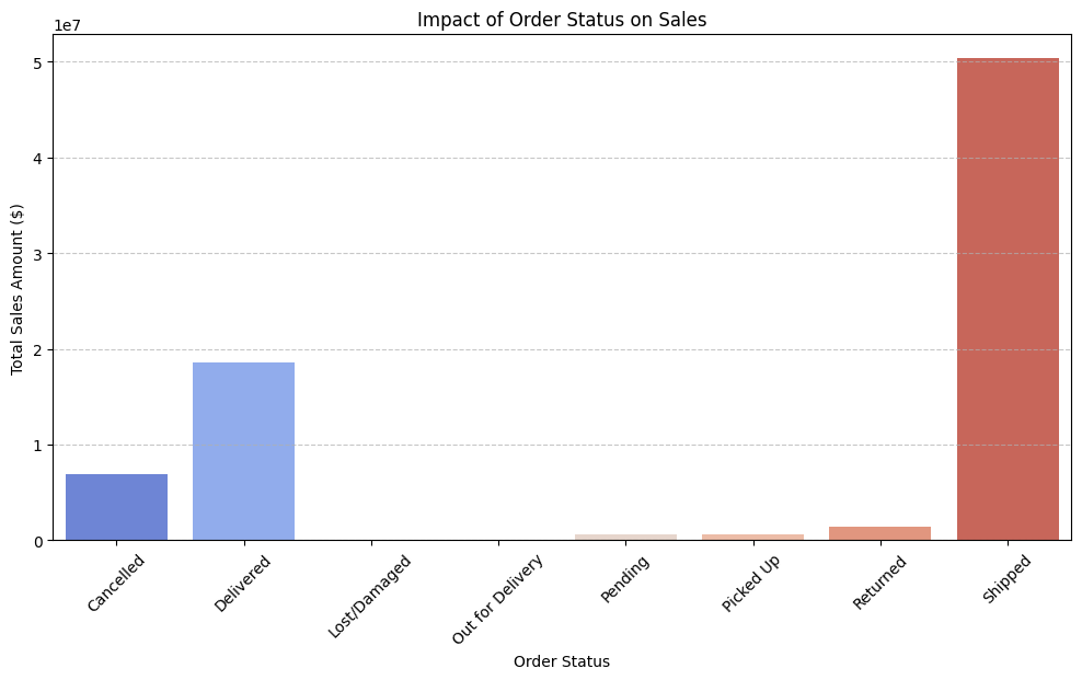
🔎 Key Insights:
1️⃣ Shipped Orders Dominate Sales
- The majority of sales (~50 million) come from Shipped orders, indicating high successful fulfillment rates.
2️⃣ Delivered Sales Are Significant
- Delivered orders contribute ~19 million, confirming a strong conversion rate from shipping to successful delivery.
3️⃣ Cancelled Orders Have Noticeable Revenue Loss
- Cancelled orders account for a significant portion (~7 million) in lost sales.
- Indicates customer dropouts or fulfillment issues affecting revenue.
4️⃣ Returned Orders Impact Sales
- Returned orders show a small but noticeable loss, suggesting product quality, incorrect shipments, or customer dissatisfaction.
5️⃣ Pending, Lost/Damaged, and Picked-Up Orders Have Minimal Impact
- These statuses represent a very small portion of total sales, meaning they are not major revenue blockers.
🚀 Actionable Recommendations:
✅ Investigate Cancelled Orders → Identify why cancellations occur and reduce lost sales.
✅ Improve Delivery Success Rate → Ensure shipped orders convert to delivered orders more efficiently.
✅ Analyze Returns → Assess why customers return products and optimize policies.
✅ Enhance Order Tracking → Ensure smooth fulfillment to reduce delays, losses, and damages.