Avocado Market Analysis

Home // AI-Powered Data Analysis

📋 Project Overview

This project leverages the Avocado dataset to uncover key insights that can drive strategic decisions for a grocery chain. By analyzing historical sales data, the project aims to address several business challenges, such as optimizing pricing strategies, forecasting demand, and understanding regional sales dynamics. It also evaluates consumer preferences by comparing conventional versus organic avocados, identifies seasonal trends for promotional campaigns, and explores untapped regional market opportunities.

The analysis showcases a comprehensive approach to data-driven decision-making, combining data cleaning, exploratory analysis, and visualization techniques. Ultimately, the goal is to transform raw data into actionable insights that support revenue growth, improved inventory management, and targeted marketing efforts.

⚙ Business Challenges

Optimizing Pricing Strategies:

How can we adjust pricing based on historical trends to maximize revenue and maintain competitive margins?

Demand Forecasting & Inventory Management:

What seasonal or regional trends affect avocado sales, and how can we forecast demand to optimize stock levels?

Product Mix & Consumer Preference Analysis:

How does the sales performance differ between conventional and organic avocados, and what does that mean for our product offerings in different regions?

Seasonal Demand Analysis for Promotional Campaigns:

Analyze seasonal patterns in avocado sales and pricing to determine optimal times for promotions or targeted discounts, ensuring inventory and marketing strategies align with demand fluctuations.

Regional Market Opportunity Analysis:

Identify underperforming regions with latent demand or emerging trends, allowing for targeted market expansion or customized marketing efforts based on regional consumer behavior.

📊 Summary of the Dataset

🗃 Key Dataset Information

Total Records: 18,249
Total Columns: 13
Time Period Covered: 2015-01-04 to 2018-03-25
Geographic Coverage: 54 regions across the United States

💲 Sales & Price Data

Date: Weekly date of observation
AveragePrice: Average price of a single avocado (USD)
Total Volume: Total number of avocados sold
PLU Codes (4046, 4225, 4770): Volume sold under each specific code
Total Bags, Small Bags, Large Bags, XLarge Bags: Number of bagged avocados sold in different sizes

🥑 Product Type

Type: Indicates whether the avocados are conventional or organic
Year: Year in which the sales data was recorded

💡 Potential Use Cases

Demand Forecasting: Predict future avocado sales based on historical volume and price
Pricing Strategy: Optimize pricing by examining trends in average price and volume sold
Regional Market Analysis: Compare performance and consumer preferences across different regions

📃 Scope of Work

📂 Data Understanding & Acquisition

Identify key data sources
Define objectives and business questions

🧹 Data Cleaning & Preprocessing

Remove duplicates and handle missing values
Ensure data consistency and integrity

🔎 Exploratory Data Analysis (EDA)

Identify trends, patterns, and outliers
Visualize relationships between key variables

🤖 Predictive Modeling

Apply forecasting or regression techniques (if applicable)
Evaluate model performance and accuracy

📊 Insights & Recommendations

Translate findings into actionable business insights
Propose strategic recommendations based on analysis

📝 Documentation & Reporting

Maintain clear records of methodologies and decisions
Present final results in an organized, stakeholder-friendly format

📈 Data Analysis Process

Data Collection & Integration

Azure SQL Data Extraction

				
					from azure.storage.blob import BlobServiceClient
import pandas as pd
import io

# 🔹 Security + networking → Shared access signature (SAS) → Blob/Container/Object → Generate SAS and connection string
STORAGE_ACCOUNT_NAME = "churndataanalysisstorage"
CONTAINER_NAME = "avocado-analysis"
BLOB_NAME = "avocado.csv"
SAS_TOKEN = "sv=2022-11-02&ss=bfqt&srt=sco&sp=rwdlacupyx&se=2026-01-09T03:06:19Z&st=2025-03-07T19:06:19Z&spr=https&sig=AbA%2B9K%2B7%2BgUCPj8x8cgHk0JTrTBUwzHtHwrRYJ6aD08%3D"  # Get this from Azure Portal

# 🔹 Create the Blob Service Client
blob_service_client = BlobServiceClient(
    account_url=f"https://{STORAGE_ACCOUNT_NAME}.blob.core.windows.net",
    credential=SAS_TOKEN
)

# 🔹 Get the blob client
blob_client = blob_service_client.get_blob_client(container=CONTAINER_NAME, blob=BLOB_NAME)

# 🔹 Download & Read as CSV
blob_data = blob_client.download_blob().readall()
df = pd.read_csv(io.BytesIO(blob_data))

df.head()

Date	AveragePrice	Total Volume	4046	4225	4770	Total Bags	Small Bags	Large Bags	type	year	region
2015-12-27	1.33	64236.62	1036.74	54454.85	48.16	8696.87	8603.62	93.25	conventional	2015	Albany
2015-12-20	1.35	54876.98	674.28	44638.81	58.33	9505.56	9408.07	97.49	conventional	2015	Albany
2015-12-13	0.93	118220.22	794.7	109149.67	130.5	8145.35	8042.21	103.14	conventional	2015	Albany
2015-12-06	1.08	78992.15	1132.0	71976.41	72.58	5811.16	5677.4	133.76	conventional	2015	Albany
2015-11-29	1.28	51039.6	941.48	43838.39	75.78	6183.95	5986.26	197.69	conventional	2015	Albany

Data Preprocessing & Cleaning

				
					# Overview
df.info()

				
					<class 'pandas.core.frame.DataFrame'>
RangeIndex: 18249 entries, 0 to 18248
Data columns (total 13 columns):
 #   Column        Non-Null Count  Dtype  
---  ------        --------------  -----  
 0   Date          18249 non-null  object 
 1   AveragePrice  18249 non-null  float64
 2   Total Volume  18249 non-null  float64
 3   4046          18249 non-null  float64
 4   4225          18249 non-null  float64
 5   4770          18249 non-null  float64
 6   Total Bags    18249 non-null  float64
 7   Small Bags    18249 non-null  float64
 8   Large Bags    18249 non-null  float64
 9   XLarge Bags   18249 non-null  float64
 10  type          18249 non-null  object 
 11  year          18249 non-null  int64  
 12  region        18249 non-null  object 
dtypes: float64(9), int64(1), object(3)
memory usage: 1.8+ MB

				
					# Convert the Date column to datetime format
df['Date'] = pd.to_datetime(df['Date'])

				
					# Check for duplicate rows
duplicate_count = df.duplicated().sum()
print(f"Number of duplicate rows: {duplicate_count}")

				
					Number of duplicate rows: 0

				
					# Standardize Column Names
df = df.rename(columns={
    'Date': 'date',
    'AveragePrice': 'average_price',
    'Total Volume': 'total_volume',
    '4046': 'plu_4046',
    '4225': 'plu_4225',
    '4770': 'plu_4770',
    'Total Bags': 'total_bags',
    'Small Bags': 'small_bags',
    'Large Bags': 'large_bags',
    'XLarge Bags': 'xlarge_bags',
    'type': 'avocado_type',
    'year': 'year',
    'region': 'region'
})

Exploratory Data Analysis (EDA)

				
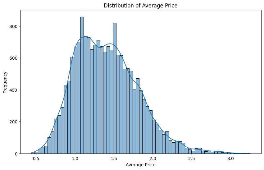
					'''Distribution of average_price'''

plt.figure(figsize=(10,6))
sns.histplot(df['average_price'],kde=True)
plt.title('Distribution of Average Price')
plt.xlabel('Average Price')
plt.ylabel('Frequency')
plt.show()

				
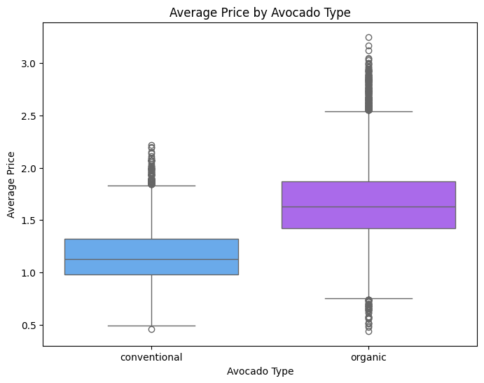
					'''Compare Average Price by Avocado Type'''

plt.figure(figsize=(8,6))
sns.boxplot(data=df, x='avocado_type', y='average_price',palette='cool')
plt.title('Average Price by Avocado Type')
plt.xlabel('Avocado Type')
plt.ylabel('Average Price')
plt.show()

				
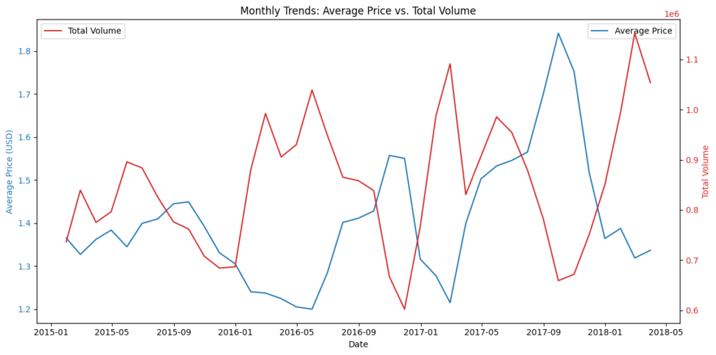
					'''Seasonal Demand Analysis Over Time'''

# Resample data by month and calculate mean of numeric columns
df_monthly = df.set_index('date').resample('M').mean(numeric_only=True)

fig, ax1 = plt.subplots(figsize=(12,6))

# Plot average_price on the primary y-axis
color = 'tab:blue'
ax1.set_xlabel('Date')
ax1.set_ylabel('Average Price (USD)', color=color)
sns.lineplot(data=df_monthly, x=df_monthly.index, y='average_price', ax=ax1, color=color, label='Average Price')
ax1.tick_params(axis='y', labelcolor=color)

# Create a secondary y-axis for total_volume
ax2 = ax1.twinx() #Create a second y-axis on the same plot, sharing the same x-axis
ax2.set_ylabel('Total Volume', color='tab:red')
sns.lineplot(data=df_monthly, x=df_monthly.index, y='total_volume', ax=ax2, color='tab:red', label='Total Volume')
ax2.tick_params(axis='y', labelcolor='tab:red')

plt.title('Monthly Trends: Average Price vs. Total Volume')
fig.tight_layout()
plt.show()

				
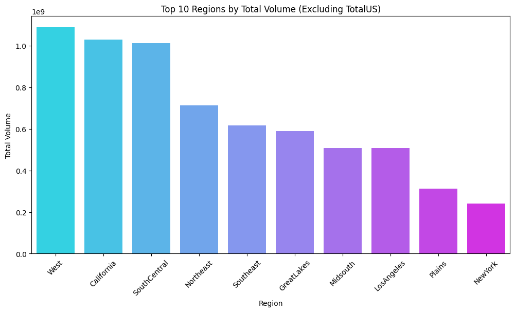
					'''Regional Analysis'''

# Remove the TotalUs to compare individual regions only
df_no_totalus = df[df['region'] != 'TotalUS']

# Aggregate total volume and average price by region (excluding TotalUS)
regional_stats_no_totalus = df_no_totalus.groupby('region').agg({
    'total_volume': 'sum',
    'average_price': 'mean'
}).reset_index()

# Sort by total volume
regional_stats_no_totalus = regional_stats_no_totalus.sort_values('total_volume', ascending=False)

# Plot top 10 regions by total volume
top_10_regions = regional_stats_no_totalus.head(10)
plt.figure(figsize=(12, 6))
sns.barplot(data=top_10_regions, x='region', y='total_volume', palette='viridis')
plt.title('Top 10 Regions by Total Volume (Excluding TotalUS)')
plt.xlabel('Region')
plt.ylabel('Total Volume')
plt.xticks(rotation=45)
plt.show()

				
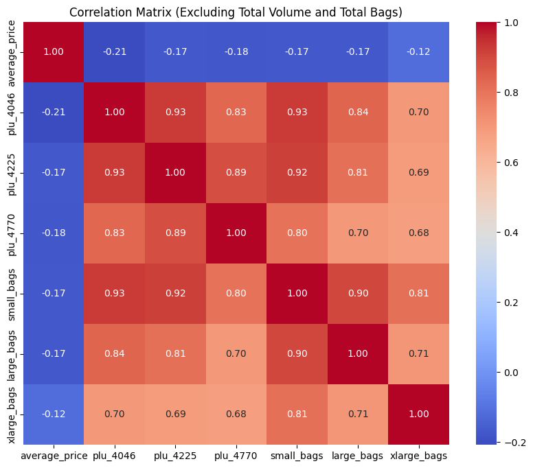
					'''Relationship Between Price & Volume'''

# Select numeric columns of interest
numeric_cols = [
    'average_price', 'plu_4046', 'plu_4225',
    'plu_4770', 'small_bags', 'large_bags', 'xlarge_bags'
]

corr_matrix = df[numeric_cols].corr()

plt.figure(figsize=(10, 8))
sns.heatmap(corr_matrix, annot=True, cmap='coolwarm', fmt='.2f')
plt.title('Correlation Matrix (Excluding Total Volume and Total Bags)')
plt.show()

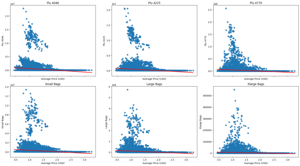
# List of interest columns
interest_cols = ['plu_4046', 'plu_4225', 'plu_4770', 'small_bags', 'large_bags', 'xlarge_bags']

# Define number of rows and columns
rows = 2
cols = 3

# Create subplots with 2 rows and 3 columns
fig, axes = plt.subplots(rows, cols, figsize=(cols * 6, rows * 5), sharex=True)

# Flatten the axes array for easy iteration
axes = axes.flatten()

# Create a regression plot for each interest column
for ax, col in zip(axes, interest_cols):
    sns.regplot(x='average_price', y=col, data=df, ax=ax, line_kws={'color': 'red'})
    ax.set_title(f'{col.replace("_", " ").title()}')
    ax.set_xlabel('Average Price (USD)')
    ax.set_ylabel(col.replace("_", " ").title())

plt.tight_layout()
plt.show()

				
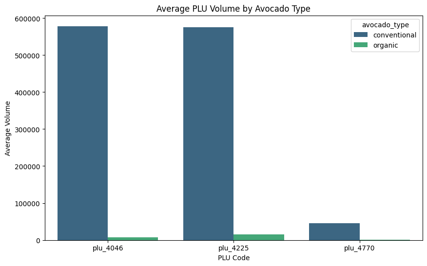
					'''Product Mix & Consumer Preference Analysis'''

# Group by avocado type and calculate the mean for selected PLU columns
avocado_mix = df.groupby('avocado_type')[['plu_4046', 'plu_4225', 'plu_4770']].mean().reset_index()

# Reshape the DataFrame for easier plotting (melt format)
avocado_mix_melted = avocado_mix.melt(id_vars='avocado_type', var_name='PLU', value_name='AverageVolume')

# Plot grouped bar chart
plt.figure(figsize=(10, 6))
sns.barplot(data=avocado_mix_melted, x='PLU', y='AverageVolume', hue='avocado_type', palette='viridis')
plt.title('Average PLU Volume by Avocado Type')
plt.xlabel('PLU Code')
plt.ylabel('Average Volume')
plt.show()

				
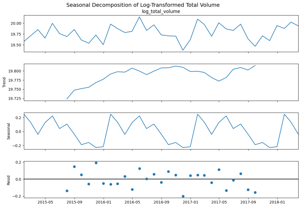
					from statsmodels.tsa.seasonal import seasonal_decompose

# Resample the data monthly, summing total volume
df_monthly_sum = df.set_index('date').resample('M').sum(numeric_only=True)

# Log transform to reduce skew
df_monthly_sum['log_total_volume'] = np.log(df_monthly_sum['total_volume'])

# Seasonal decomposition on the log-transformed volume
decomposition = seasonal_decompose(df_monthly_sum['log_total_volume'], model='additive', period=12)

# Increase figure size for better visibility
fig = decomposition.plot()
fig.set_size_inches(12, 8)
plt.suptitle('Seasonal Decomposition of Log-Transformed Total Volume', fontsize=14)
plt.show()

📡 Predictive Modeling

Random Forest Regression

				
					'''Feature Engineering'''

# Convert date to ordinal
df['date'] = pd.to_datetime(df['date'])  # ensure it's datetime
df['date_ordinal'] = df['date'].apply(lambda x: x.toordinal())

# Encode avocado type (binary)
df['type_encoded'] = df['avocado_type'].map({'conventional': 0, 'organic': 1})

# One-hot encode region
df_encoded = pd.get_dummies(df, columns=['region'])

# Select features (X) and target (y)
feature_cols = [
    'date_ordinal',        # numeric representation of date
    'average_price',       # price feature
    'type_encoded',        # avocado type (conventional vs. organic)
    'year'                 # year can also be a feature
]

# Add region dummies to feature list
region_cols = [col for col in df_encoded.columns if col.startswith('region_')]
feature_cols.extend(region_cols)

X = df_encoded[feature_cols]
y = df_encoded['total_volume']

'''Train-Test Split'''

from sklearn.model_selection import train_test_split

# 80% training, 20% testing
X_train, X_test, y_train, y_test = train_test_split(X, y, 
                                                    test_size=0.2, 
                                                    random_state=42)

'''Model Training & Prediction'''

from sklearn.ensemble import RandomForestRegressor

# Initialize Random Forest
rf = RandomForestRegressor(n_estimators=100, random_state=42)
rf.fit(X_train, y_train)

# Predict on test set
y_pred = rf.predict(X_test)

'''Model Evaluation'''

from sklearn.metrics import mean_absolute_error, mean_squared_error
import numpy as np

mae = mean_absolute_error(y_test, y_pred)
mse = mean_squared_error(y_test, y_pred)
rmse = np.sqrt(mse)

print("MAE:", mae)
print("RMSE:", rmse)

				
					MAE: 68034.06354476715
RMSE: 510651.0141577325

💡 Insights & Recommendations

✅ Optimizing Pricing Strategies

💡Insights

- Avocado prices generally fall within a moderate range, suggesting consumers are price-sensitive above certain thresholds.
- A negative relationship between price and volume indicates that higher prices can reduce sales, though organic avocados can sustain a premium due to perceived quality.

🎨Recommendations

- Price Positioning: Maintain competitive pricing for conventional avocados around the observed sweet spot to maximize volume.
- Premium Strategy: Capitalize on organic avocados’ higher price tolerance in regions where demand remains strong despite elevated prices.
- Ongoing Monitoring: Regularly evaluate price elasticity using updated data to refine pricing decisions.

✅ Demand Forecasting & Inventory Management

💡Insights

- Time-series analysis shows recurring patterns, with certain periods experiencing higher demand.
- A Random Forest model with lag features significantly improved forecast accuracy, indicating that historical sales trends are predictive of future volume.

🎨Recommendations

- Seasonal Stocking: Increase inventory during identified peak months to prevent stockouts.
- Refined Forecasts: Continue enhancing the Random Forest approach with additional features (e.g., promotions, holidays) and consider advanced models (SARIMA, Prophet) to capture seasonality.
- Safety Stock Policies: Leverage forecast outputs to set optimal reorder points, balancing cost and service levels.

✅ Product Mix & Consumer Preference Analysis

💡Insights

- Conventional avocados dominate total volume, but organic avocados consistently command higher prices, indicating distinct consumer segments.
- Certain product codes (PLUs) are more popular, contributing disproportionately to total sales.

🎨Recommendations

- Inventory Prioritization: Allocate shelf space to high-volume PLUs while maintaining a curated organic selection in markets that support premium pricing.
- Targeted Promotions: Tailor deals to the most popular product codes, reinforcing consumer loyalty and boosting overall sales.
- Consumer Segmentation: Identify markets where organic offerings are in higher demand and focus marketing efforts there.

✅ Seasonal Demand Analysis for Promotional Campaigns

💡Insights

- The data reveals cyclical demand spikes and dips throughout the year.
- Price changes and promotional timing can significantly influence weekly or monthly sales volumes.

🎨Recommendations

- Timed Discounts: Offer promotions during lower-volume months to stimulate demand and maintain steady sales.
- Event-Driven Marketing: Leverage known seasonal or holiday periods that correlate with demand surges for targeted campaigns.
- Bundling Strategies: Combine avocados with complementary products (e.g., chips, salsa) during peak demand seasons to drive incremental revenue.

✅ Regional Market Opportunity Analysis

💡Insights

- Certain regions consistently lead in total volume, indicating strong consumer demand and established distribution networks.
- Other regions show moderate but growing sales, suggesting potential for targeted expansion.

🎨Recommendations

- Resource Allocation: Prioritize high-volume regions for marketing and supply chain investments.
- Benchmarking: Compare regional performance to national aggregates to identify underperforming areas with untapped potential.
- Localized Strategy: Adapt product mix and promotional tactics to each region’s consumer preferences and price sensitivity.

📑 Reporting (Power BI)

DAX Snippet

				
					Total Volume = sum(avocado[sold volume])

Total PLU = 
CALCULATE(
    [Total Volume],
    ABS(avocado[Sold Types] IN {"4046", "4225", "4770"}
)
)

Total Bags = 
CALCULATE(
    [Total Volume],
    NOT avocado[Sold Types] IN {"4046", "4225", "4770"}
)

Avg. Price = AVERAGE(avocado[AveragePrice] )

YoY Growth = 
VAR CurrentYearValue = [Total Volume]
VAR PreviousYearValue = CALCULATE(
    [Total Volume], 
    SAMEPERIODLASTYEAR('DateTable'[Date])
)
RETURN
IF(
    ISINSCOPE('DateTable'[Year]),  // Ensures calculation only applies at the Year/Quarter level
    IF(
        NOT(ISBLANK(PreviousYearValue)) && NOT(ISBLANK(CurrentYearValue)), 
        DIVIDE(CurrentYearValue - PreviousYearValue, PreviousYearValue, BLANK()), 
        BLANK()
    ), 
    BLANK()  // Returns BLANK for the Total Row
)

Avocado Market Analysis

📂 Table of Content

📋 Project Overview

⚙ Business Challenges

📊 Summary of the Dataset

📃 Scope of Work

📈 Data Analysis Process

Data Collection & Integration

Data Preprocessing & Cleaning

Exploratory Data Analysis (EDA)

📡 Predictive Modeling

Random Forest Regression

💡 Insights & Recommendations

📑 Reporting (Power BI)

Quick Links

Get In Touch

Avocado Market Analysis

📂 Table of Content

📋 Project Overview​

⚙ Business Challenges

📊 Summary of the Dataset​

📃 Scope of Work

📈 Data Analysis Process

Data Collection & Integration

Data Preprocessing & Cleaning

Exploratory Data Analysis (EDA)

📡 Predictive Modeling

Random Forest Regression

💡 Insights & Recommendations

📑 Reporting (Power BI)

Quick Links

Get In Touch

📋 Project Overview

📊 Summary of the Dataset