📈 Exploratory Data Analysis (EDA)
Exploratory Data Analysis (EDA)
Which income levels and education backgrounds are most associated with higher divorce rates?
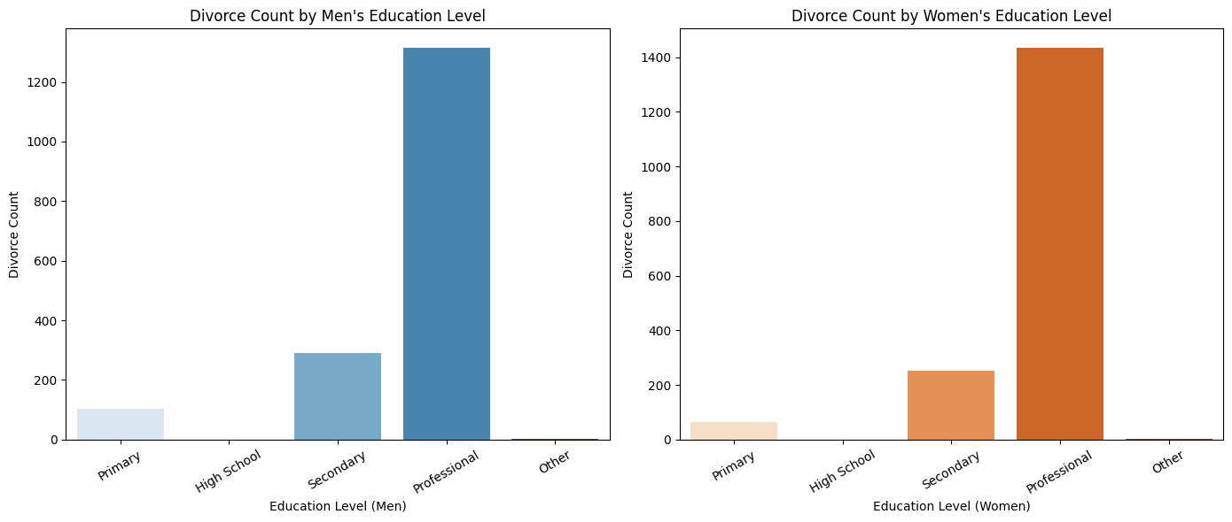
Higher divorce rates are observed among professionally educated individuals, especially women, possibly due to career demands and financial independence. In contrast, lower-educated individuals show fewer divorces, potentially influenced by traditional family values or economic dependence.
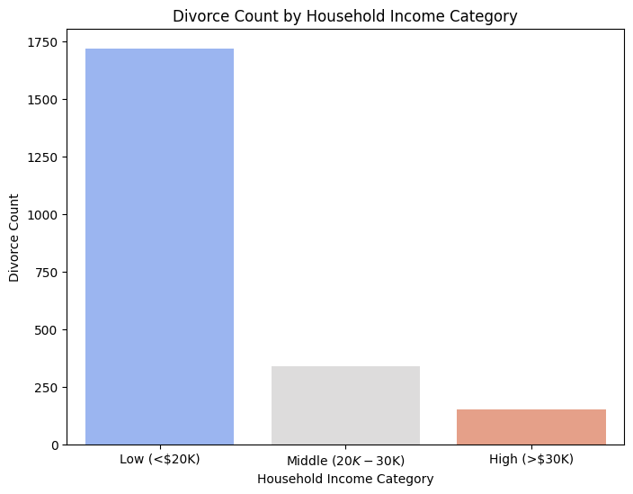
Divorce rates are significantly higher among low-income households, suggesting financial instability as a major factor in marital breakdowns. Higher-income groups experience fewer divorces, indicating better financial security may contribute to marriage stability.
Are there common patterns in marriage duration before divorce?
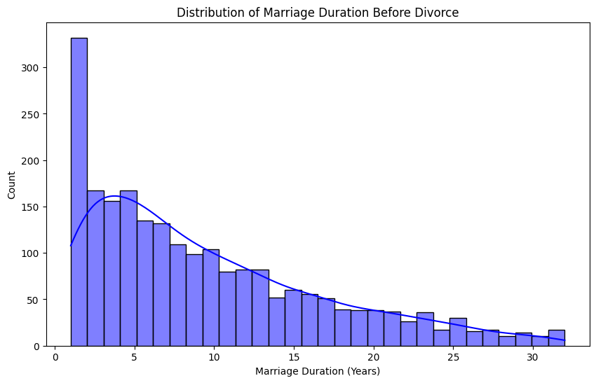
This histogram shows the distribution of marriage duration before divorce. The data is right-skewed, indicating that most divorces happen within the first few years of marriage, with a sharp decline as the duration increases. The highest frequency is observed at very short durations (0-5 years), reinforcing the trend that early divorces are more common. Longer marriages before divorce are much less frequent. This suggests that if a couple stays together beyond the early years, their chances of long-term stability increase.
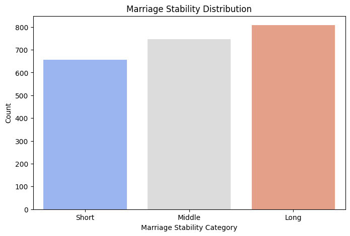
This bar chart illustrates the distribution of marriage stability categories. "Short" marriages (less than 5 years) account for a significant portion of divorces, but "Middle" (5-10 years) and "Long" (10+ years) durations also have substantial divorce counts. The trend suggests that while many divorces occur early, a considerable number also happen after a decade, indicating that long-term marital challenges still contribute to divorce.
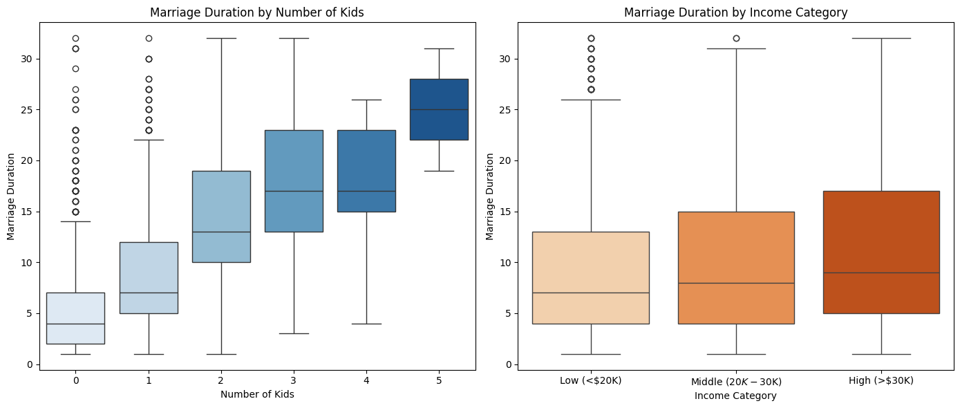
The left boxplot shows that marriage duration tends to increase with the number of children, indicating that couples with more kids are likely to stay married longer. The right boxplot reveals that income level has a weaker correlation with marriage duration, as all income groups show similar distributions, though higher-income couples exhibit slightly longer marriages on average.
Does household income affect marriage stability?
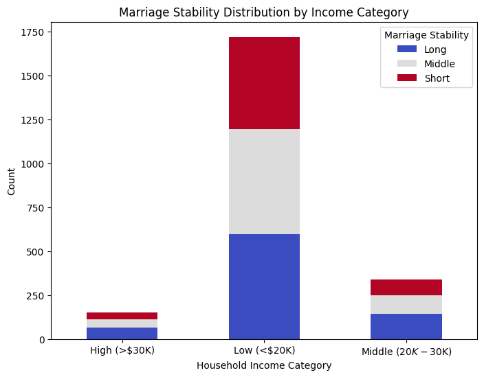
The majority of divorces occur in the low-income category ($30K) tend to have longer marriages before divorce, suggesting financial stability may contribute to longer marriage durations.
This bar chart illustrates the distribution of marriage stability categories. "Short" marriages (less than 5 years) account for a significant portion of divorces, but "Middle" (5-10 years) and "Long" (10+ years) durations also have substantial divorce counts. The trend suggests that while many divorces occur early, a considerable number also happen after a decade, indicating that long-term marital challenges still contribute to divorce.
The left boxplot shows that marriage duration tends to increase with the number of children, indicating that couples with more kids are likely to stay married longer. The right boxplot reveals that income level has a weaker correlation with marriage duration, as all income groups show similar distributions, though higher-income couples exhibit slightly longer marriages on average.
Do income differences between partners correlate with divorce?
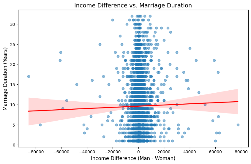
The scatter plot shows a weak positive correlation between income difference and marriage duration, suggesting that income disparity between spouses has minimal impact on how long a marriage lasts. Most divorces occur among couples with small income differences, while extreme income gaps (both high and low) do not significantly alter marriage duration trends.
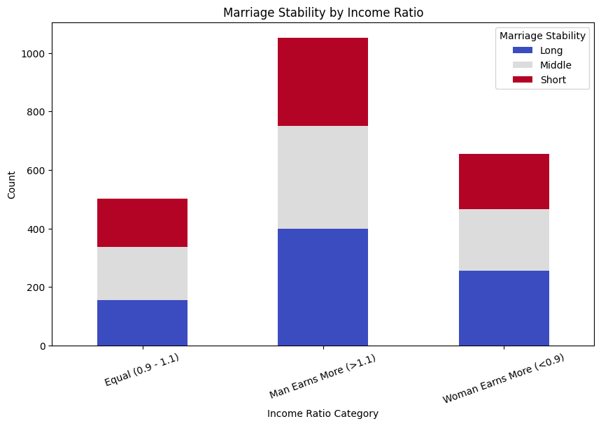
This chart illustrates the relationship between income ratio and marriage stability. Couples where the man earns significantly more (>1.1 ratio) have the highest divorce count, with a notable portion categorized as short marriages. In contrast, equal-income couples (0.9-1.1 ratio) and those where the woman earns more (<0.9 ratio) show relatively fewer short marriages, indicating that financial balance or the woman having a higher income may contribute to longer marriage durations.
Are younger or older couples more likely to divorce?
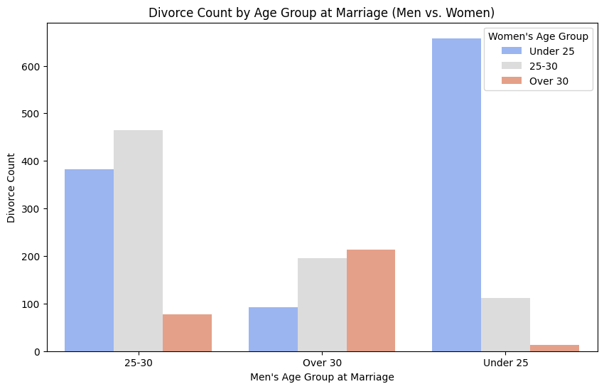
This chart shows divorce counts based on the age groups at marriage for both men and women. Men who married under 25 have the highest divorce rates, especially when their wives were also under 25. Divorce rates remain high for men who married at 25-30, particularly with partners in the same age group. However, divorces decrease significantly for men who married over 30, indicating greater marriage stability at later ages. Overall, younger marriages tend to have higher divorce rates, and couples of similar ages experience more divorces than those with larger age gaps.
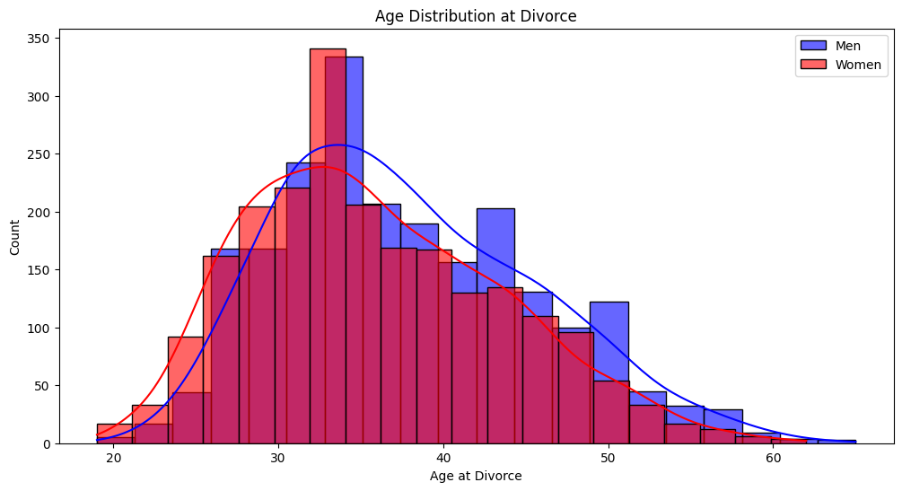
This histogram shows the distribution of ages at divorce for men and women. The peak divorce age for women is slightly lower than for men, with most divorces occurring in the late 20s to early 30s for both genders. However, men tend to have a wider distribution, with divorces occurring more frequently at older ages compared to women.
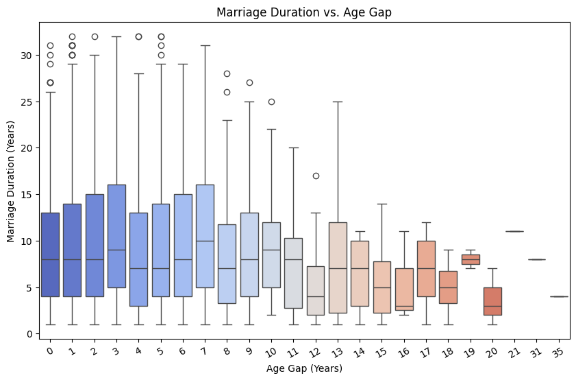
This boxplot illustrates the relationship between age gap and marriage duration. Marriages with smaller age gaps (0-5 years) tend to last longer, with higher median durations and more variability. As the age gap increases beyond 10 years, marriage duration generally decreases, with more compact distributions and lower medians, suggesting that larger age differences may be linked to shorter marriages.
Key Insights:
🤖 Machine Learning
Data Preparation & Feature Selection
Model Selection & Training
Visualizations
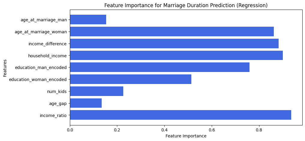
This feature importance chart for the Marriage Duration Prediction Model (Regression) shows that income ratio has the highest impact on predicting marriage duration, followed by household income and education levels. Age at marriage and income difference also play significant roles, while age gap has a relatively lower influence. These insights suggest that financial and educational factors strongly impact marriage longevity. Let me know if you need further refinement!
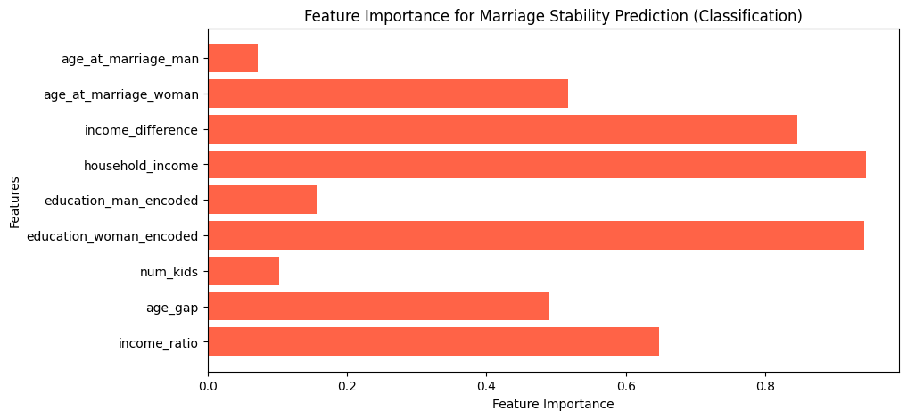
This feature importance chart for the Marriage Stability Prediction Model (Classification) highlights that education level (especially women's education), household income, and income difference are the strongest predictors of marriage stability. Age gap and income ratio also contribute significantly, while age at marriage for men and number of kids have a lower impact. These findings suggest that financial and educational differences strongly influence whether a marriage lasts.